Most people are familiar with compressing data files so that they require less memory and they are easier to send electronically. Similar concepts are popular with process data historians. Data compression for process historians involves reducing the number of data points that are stored, while trying to not affect the quality of the data.
Compression can be accomplished using one of several algorithms (swinging door, Box Car Back Slope). Each algorithm uses some criteria to eliminate data between points where there is constant change (slope), within some tolerance.
The main drivers for compression are disk space, and network traffic or data retrieval speed. The goal of compression is to remove data that is “unimportant”. The proponents of compression make convincing arguments, like the shape of the graph is still the same. However, there are several drawbacks to data compression for process historians.
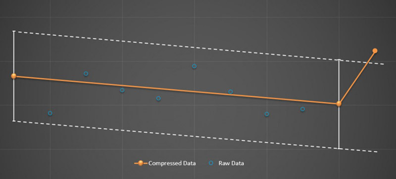
Process data compression algorithm. Here, 3 data points are stored to represent the trend created by 11 raw data points.
Data Compression Downsides
Data is LOST Forever
The first, and most important, disadvantage of compression is the permanent loss of data. When you erase data, you are relying on interpolation between archived points. You can’t go back later when you find out that it actually was important and recover the lost data.
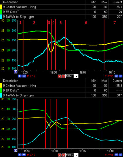
Consider the multiple effect evaporator example in Figure 2 that shows a graphical comparison between raw data recorded every 5 sec. (top graph) and compressed data (bottom graph). The frequency of compressed data is variable, but there is an average of one point per minute, which is typical where data compression is set too high when using percent deviation of absolute change or a slope algorithm for compression.
Effect of interpolation
The trends look similar, but when you investigate more closely there are some differences at critical points. Both graphs show a rapid drop in vacuum (yellow) at the start of stage 3. The compressed data indicates that the temperature (green) started rapidly decreasing at the same time as the vacuum. However, the raw data shows that the temperature didn’t shift much until the vacuum reached its minimum level 30 seconds later. This difference can lead to a completely different conclusion about the root cause of the vacuum drop because it is critical to know the correct sequence of events when problem solving. The actual cause, insufficient condensate removal, is confirmed by analyzing the raw data in stages 3 and 4. In this situation the problem was isolated correctly and the field search was narrowed to a 20 foot section of pipe and the pump. The actual problem turned out to be a leaky seal at the pump. The compressed data could have pointed to something wrong in another part of the plant.
Looking for a higher-performance historian? Get an enterprise plant data historian at half the cost.
Compression Changes Statistics
By compressing the data, you lose fidelity. Although compression can maintain the general shape of the data trend, statistical properties such as mean and standard deviation are different. Therefore, statistics from compressed data can be misleading. Variability has a significant impact on cost and quality, so it is important to accurately calculate the variance (or standard deviation).
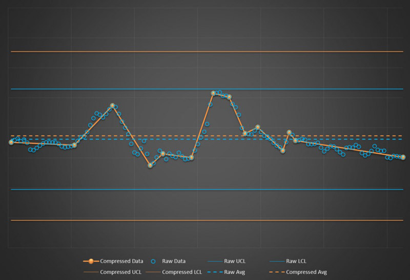
Compression will also affect any other calculations that are based on the statistics. For example, control chart limit calculations will be different with compressed data. Typically, you will have a larger standard deviation for compressed data, so the control limits will also increase. As you can see in Figure 3, the average is different and the control chart limits are much wider for the compressed data set. This could cause you to misinterpret future events.
Effect of data compression on control chart limits
Creates More Administrative Work
With appropriate compression settings, the effects can be minimized, but this is easier said than done. Optimizing compression settings requires evaluation on a per-point basis because there isn’t a standard compression that will work for all measurements. When you have thousands of tags, it is highly unlikely that every tag has the ideal compression settings because compression settings depend on the type of sensor, accuracy of the measurement, and operating range of the variable, to name a few.
Consider a temperature measurement that has a range of possible values from 50 to 150 ˚F but typical values during normal operation are 95-97 ˚F and the process is very temperature sensitive. If this point is set up with a 1% compression deviation, you could be deleting values that don’t change by more than one degree. However, most temperature sensors are accurate to fractions of a degree. These changes should be captured and saved, especially where the temperature is being controlled so you can monitor the control loop.
Alternatives To Data Compression For Process Historians
Instead of compression, it’s possible to address the data retrieval speed in a different way. dataPARC’s Performance Data Engine creates a separate archive to improve retrieval and trending for large time periods, generally periods > 2 days. This gives you the best of both worlds, no data is deleted, and the concern about archive performance is alleviated. When zoomed in on short time periods, there are fewer data points so all of the raw data can be displayed. Your original data will always be available when needed, so why would you want to compromise for performance when you don’t have to?
For more information, and examples of how “lossless” data can work in an actual manufacturing process, check out our post about getting high-performance data from your PIMS.
Digital Transformation Roadmap
Download our Digital Transformation Roadmap and learn what steps you can take to achieve data-driven success in manufacturing.