When Your Historian Data Doesn’t Add Up – Literally

Data historian compression is a fact of life in manufacturing. Configuring it well keeps storage costs manageable and systems running efficiently, but when settings aren’t matched to how the data is actually used, the consequences can show up in unexpected places. In this post, we walk through a real-world case where historian configuration caused two reports pulling from the same data source to produce different numbers, what was behind it, and how it was resolved. If your historian settings have been on autopilot since initial setup, this one is worth a read.

When a report is right and an automated pull of the same data is wrong, the obvious assumption is that something broke. But what if both are technically correct, just not at the same moment in time?

That’s the kind of problem that doesn’t show up in an error log. It shows up in an accounting reconciliation, with a frustrated finance team staring at a discrepancy they can’t explain and thousands of pounds of inventory that seem to have disappeared.

Historian configuration, compression settings, scan rates, keep-alive intervals, these are all settings that are easy to set once and forget. But the decisions made at setup have a direct impact on data accuracy, and in process-heavy industries where calculations stack on top of calculations, small configuration gaps can surface as surprisingly large real-world errors.

This is the story of one of those situations, what caused it, and what it reveals about how historian settings should be thought about from the start.

The Case of the Disappearing Inventory

A few days after an automated report was set up, the accounting team flagged that the numbers didn’t match the existing report and refused to use them until they did. On the surface, this was puzzling. The automation was pulling values the same way as the manual report, from the same data source. The discrepancies were small; the largest was about 0.13%, and most were 0.03% or lower. But when the tanks in question hold hundreds of thousands or millions of pounds of product, even a fraction of a percent can translate to thousands of pounds of missing inventory. That’s not something accounting is willing to overlook.

The first clue came when re-running the automation produced values that suddenly aligned with the existing report. That pointed to a timing issue. The automated pull was running at 6:30 AM,  30 minutes after the 6:00 AM snapshot it was targeting. Most of the inputs to the report were calculations that were not historized, meaning they ran on demand each time the report was opened. If someone pulled up the report manually after the automation had already run, the underlying data could have shifted in the window between the two.

That was the hypothesis. Proving it required a closer look at how the historian was configured.

How Historians Handle Data

To understand what went wrong, it helps to understand how process historians store data in the first place.

In an ideal world, every variable would be recorded every millisecond. In practice, that’s not realistic. Most control systems can’t handle that volume of requests while still doing their primary job of controlling the process. Even if they could, the storage costs would become significant very quickly.

So, historians make assumptions. Data is sampled at a fixed rate, often every second, sometimes faster, sometimes slower. But the effective sampling rate is really governed by the slowest link in the chain. In an OPC DA/UA setup, for example, it’s typically the OPC server’s scan rate that sets the ceiling regardless of how often the historian requests values.

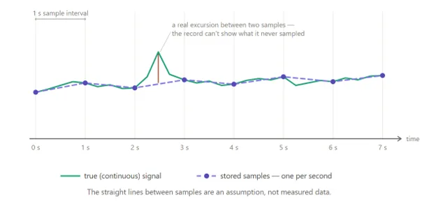
This graph shows how a real excursion between two samples may not show up in the data depending on compression settings.

Even with reasonable sampling rates, storing every data point creates a volume problem. A tank level that barely moves for hours still generates thousands of data points, most of which are near-identical or pure noise. To address this, almost all historians use compression algorithms. The details vary, but the goal is the same: capture the shape of the data accurately while storing as few points as possible.

At its most basic, compression works by checking whether the current value has deviated from the last recorded point by more than a defined threshold. If it hasn’t, the point is discarded. Values between recorded points are assumed to be linear, a reasonable approximation, but an approximation nonetheless.

One more consideration: what happens when data goes completely flat for an extended period? Most historians include a setting to force a point to be written even when no deviation has occurred, often called a keep-alive point. In dataPARC, this is the Maximum History Intervals setting. If no deviation-triggering point has been recorded within that time window, the current raw value is committed to history regardless.

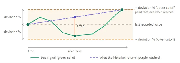
With a deviation percentage enabled, this image shows what the error could be between points while the value alternates but stays within the deviation percentage.

These are all reasonable engineering tradeoffs. But they create conditions where, depending on when you ask for a value, you might get a different answer.

How Compression Settings Created a Timing Problem

With the general mechanics of historian compression in mind, the root cause of the discrepancy becomes clearer.

The report in question was calculating tank inventories using a formula along the lines of:

Inventory = A × Level × (B – Temperature)

Where A and B are just various constants for thank volume and density correction together. The tank level tags had consistent, frequent data, often at least one recorded point per minute, sometimes several per second. The temperature tags, however, were a different story. Temperatures in these tanks were stable and slow-moving, which meant they rarely triggered the deviation threshold. As a result, the only points being committed to history for those tags were the keep-alive points. These were written once per hour at the Maximum History Intervals default setting. Here’s where the timing issue surfaces. When the automated pull ran at 6:30 AM requesting the 6:00 AM value, the most recent recorded temperature point may have been from 5:15 AM or earlier. With no bracketing point on the other side of 6:00 AM yet written, the historian had no choice but to hold the last known value forward, effectively treating a continuous variable like a state tag.

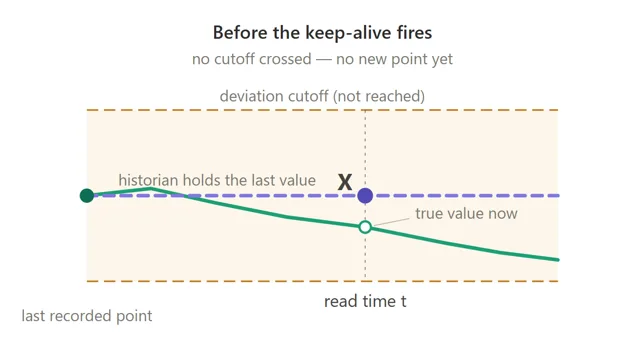
This trend illustrates how a small deviation within the deviation cutoff meant that a keep-alive value was reached and placed rather than the true value, as it was within the deviation threshold.

When the report was later opened manually, the picture had changed. By that point, the next keep-alive point had been written, giving the historian a point on both sides of 6:00 AM to interpolate between. The interpolated value at 6:00 AM shifted, sometimes by enough to move a tank inventory by thousands of pounds and suddenly the two numbers no longer matched.

The data wasn’t wrong in either case. It was just a different answer to the same question, asked at two different moments in time.

The Configuration Fix That Solved the Discrepancy

The fix itself was straightforward. By lowering the Maximum History Intervals setting on the temperature tags from one hour to ten minutes, the keep-alive points were written much more frequently. This meant that by 6:10 AM at the latest, a bracketing point existed on both sides of the 6:00 AM snapshot and the interpolated value was stable regardless of when the report was pulled.

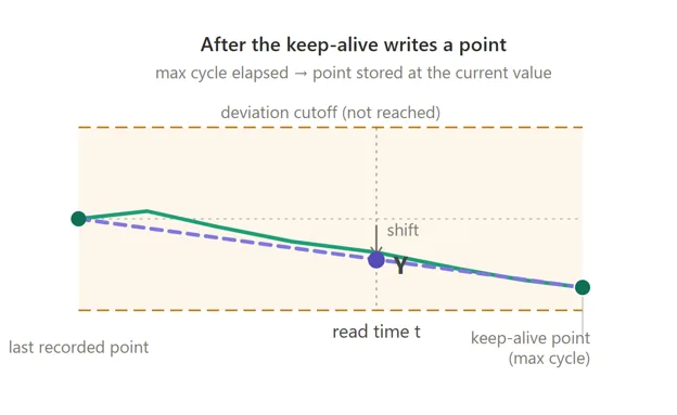
The trend indications shortening the keep-alive value helps more accurately estimate the true value at the time of the report.

The automated pull and the manual report now agreed. The accounting team had numbers they could trust.

It’s worth noting that this fix didn’t require changes to the compression deviation setting, the scan rate, or anything else in the historian configuration. The data was being collected accurately all along; the issue was simply that the keep-alive interval was too wide for a use case that required consistent, time-sensitive reads.

This is a good example of why historian configuration deserves to be thought about in terms of how the data will actually be used, not just how much storage needs to be conserved. A one-hour keep-alive is a perfectly reasonable default for many tags. For tags feeding time-critical calculations that are read on a fixed schedule, it is not.

Are Your Historian Settings Actually Matched to How You Use Your Data?

Fixing the Maximum History Intervals resolved the immediate problem. But stepping back, it surfaced a more important question: were the historian settings appropriate for what the data was being used for?

The tags in question had a compression deviation setting of 1%. That means any change smaller than 1% of the tag’s range is discarded and not recorded to history. For a tank holding 10 million pounds of material, a 1% deviation threshold represents 100,000 pounds of potential uncertainty in any given recorded value, far larger than the thousands-of-pounds discrepancy that triggered the investigation in the first place.

In practice, compression error rarely reaches its theoretical maximum. Noise tends to be distributed in both directions, and errors across multiple input tags can partially cancel each other out in a calculation. But in a worst-case scenario where all input tags drift to their individual deviation limits simultaneously and in the same direction, the cumulative error in a tank inventory calculation could reach into the hundreds of thousands of pounds.

This isn’t an argument that 1% deviation is always the wrong setting. It’s an argument that the setting should be a conscious decision tied to how the data is used. If a 1% swing in a level reading is operationally meaningless, noise within the sensor’s own accuracy limits, then 1% is a reasonable and storage-efficient choice. If that same 1% represents an inventory discrepancy that accounting needs to track and report on, a different conversation needs to happen.

The question to ask is not “what deviation setting keeps my disk usage manageable?” but “what level of uncertainty am I willing to accept in the decisions this data supports?”

Why Historian Tag Configuration Deserves More Attention Than It Gets

Historian tag configuration is one of those tasks that is easy to underestimate. The number of tags to configure at even a mid-sized facility can run into the thousands. Larger operations may have tens of thousands, or more. Each tag has its own data source, update rate, compression characteristics, and downstream use cases, and what makes sense for one tag may be completely wrong for another.

The results of a well-configured historian are largely invisible. Data flows, reports run, calculations produce consistent results, and nobody thinks much about it. The results of a poorly configured historian tend to be more visible,  but often only when something downstream breaks, like an inventory reconciliation that doesn’t close.

Too little compression and disk usage grows unchecked, generating storage costs and potentially degrading system performance as the historian processes meaningless noise. Too much compression and the data loses its value, reduced to flat lines punctuated by keep-alive points that tell you little about what actually happened between them.

There is no universal right answer. But there is a useful starting point: identify the primary business cases for the data being historized, and let those drive the configuration decisions. If the data feeds a financial reconciliation process, treat it accordingly. If it feeds a control loop optimization, the requirements are different. If it feeds both, the more demanding use case should set the standard.

Data historian compression configuration is not a one-time task. Processes change, instrumentation gets updated, and new use cases emerge for data that was originally collected for something else. Periodic review of tag settings, even a targeted audit of the tags feeding critical calculations, can have a meaningful impact on data quality and the business decisions that depend on it.